Power Meter Calibration: Traceable Measurements from DC to 110 GHz

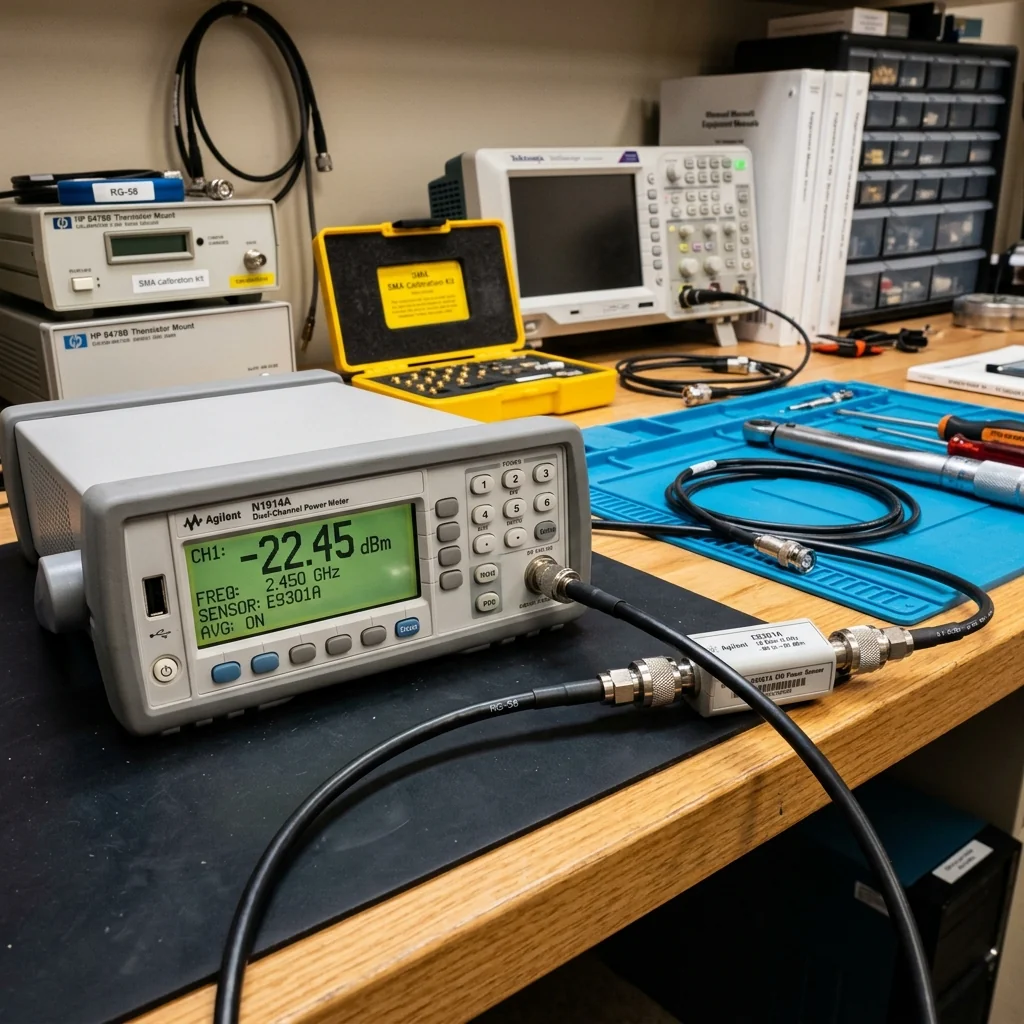
Every RF measurement ultimately traces back to power. S-parameters, gain, noise figure, EVM: they are all derived from or validated against power measurements. If your power meter is wrong, everything downstream of it is wrong. The challenge is that RF power measurement accuracy degrades with frequency. A thermocouple sensor that delivers ±0.5% uncertainty at 1 GHz may produce ±5% uncertainty at 50 GHz and ±15% at 110 GHz. Maintaining traceable, quantified measurement uncertainty across the full spectrum from DC to 110 GHz requires understanding the physics of power sensors, the mathematics of calibration factors, and the discipline of a calibration chain that connects your bench instrument to a national metrology institute.

Power Sensor Technologies

Three sensor technologies dominate RF power measurement, each with distinct operating principles and frequency-dependent performance characteristics.

Thermocouple Sensors

A thermocouple power sensor absorbs RF energy in a thin-film resistive load and measures the resulting temperature rise. The temperature difference between the load and a reference junction produces a DC voltage proportional to the absorbed RF power. Thermocouple sensors are true RMS detectors: they respond to the average power regardless of waveform shape, modulation, or crest factor. This makes them the preferred choice for measuring modulated signals like OFDM, CDMA, and pulsed radar waveforms.

The primary limitation is sensitivity. Thermocouple sensors typically have a noise floor of -30 to -35 dBm, which restricts their use to moderate and high power levels. At millimeter-wave frequencies, the internal mismatch of the sensor increases, raising the VSWR and reducing the coupling efficiency.

Diode Sensors

Diode sensors use a Schottky barrier diode to rectify the RF signal. Below the square-law region (approximately -20 dBm), the rectified DC voltage is proportional to the square of the RF voltage, which is proportional to power. Above -20 dBm, the diode enters its linear region, and corrections must be applied based on a calibration table.

Diode sensors offer much higher sensitivity than thermocouples, with noise floors of -60 to -70 dBm. However, they are waveform-dependent above the square-law region: the measured power depends on the signal's peak-to-average ratio. Modern "wide dynamic range" diode sensors combine a diode path and a resistive path to maintain accuracy from -60 to +20 dBm.

Parameter	Thermocouple	Diode (CW)	Diode (Wide DR)	Waveguide Calorimeter
Frequency Range	DC to 50 GHz	10 MHz to 110 GHz	10 MHz to 50 GHz	DC to 110 GHz
Dynamic Range	-30 to +20 dBm	-70 to +20 dBm	-60 to +20 dBm	-10 to +30 dBm
Waveform Dependence	None (true RMS)	Above -20 dBm	Corrected	None (true RMS)
Measurement Speed	Slow (100 ms)	Fast (10 μs)	Moderate (1 ms)	Very slow (10 s)
Best Accuracy	±1-3%	±3-5%	±3-5%	±0.5-1%

Calibration Factor: What It Actually Means

The calibration factor (CF) of a power sensor is the ratio of the power absorbed by the sensor to the power incident on the sensor. It accounts for the sensor's internal mismatch loss and any frequency-dependent absorption inefficiency. A perfect sensor has CF = 100% (or 0 dB). A real sensor at 40 GHz might have CF = 92%, meaning it absorbs only 92% of the incident power. The power meter firmware divides the raw measurement by the CF to report the correct incident power.

CF values are determined at a calibration laboratory by comparing the sensor under test to a reference standard whose power absorption is known to national metrology institute accuracy. For coaxial sensors, the calibration laboratory uses a precision power reference output from the power meter itself (a 50 MHz, 1 mW reference oscillator) to set the zero-frequency calibration, then applies frequency-dependent corrections from a transfer standard.

Mismatch Uncertainty: The Dominant Error Term

Above 10 GHz, mismatch uncertainty is typically the largest contributor to the total measurement uncertainty budget. Mismatch occurs because neither the source nor the sensor has a perfect 50 Ω (or waveguide characteristic) impedance. The interaction between the source reflection coefficient (Γ_S) and the sensor reflection coefficient (Γ_L) creates a standing wave that modulates the power delivered to the sensor.

The mismatch uncertainty is bounded by:

U_mismatch = ±20 × log10(1 + |Γ_S| × |Γ_L|) dB (worst case)

For a source with VSWR 1.5:1 (|Γ_S| = 0.2) and a sensor with VSWR 1.3:1 (|Γ_L| = 0.13), the mismatch uncertainty is ±20 × log10(1 + 0.026) = ±0.22 dB. At 90 GHz, where sensor VSWR might be 2.0:1, the mismatch uncertainty grows to ±0.82 dB, dominating the entire error budget.

Reducing Mismatch Uncertainty

• Precision adapters and transitions: use the highest quality waveguide-to-coaxial adapters with specified VSWR at the measurement frequency.
• Fixed attenuator pads: inserting a 6 or 10 dB precision attenuator between the source and sensor improves the effective source match at the cost of reduced power reaching the sensor.
• Measure and correct: if both Γ_S and Γ_L are known in magnitude and phase (from VNA measurements), the exact mismatch correction can be calculated, reducing the uncertainty to the uncertainty of the VNA measurement itself.

The NIST Traceability Chain

Traceable measurement means that every instrument in the measurement chain can be linked through an unbroken series of comparisons back to a national measurement standard. For RF power, the traceability chain in the United States flows from:

1. NIST Primary Standard: a microcalorimeter that measures RF power by comparing the heating effect of RF energy to the heating effect of a known DC power. This primary standard achieves uncertainties of ±0.1% at low frequencies and ±1% at millimeter-wave bands.
2. Transfer Standard: a secondary power sensor calibrated directly against the NIST primary standard. NIST issues a calibration report with CF values and uncertainties at each calibrated frequency.
3. Working Standard: the calibration laboratory's reference sensor, calibrated against the transfer standard. This is the sensor used to calibrate customer sensors.
4. Device Under Test: the customer's power sensor, calibrated against the working standard by direct comparison.

Each step in the chain adds uncertainty. A customer sensor calibrated four levels below the NIST primary standard accumulates the uncertainties of all intermediate comparisons. This is why RF Essentials recommends using the shortest traceability chain possible for critical measurements, and why the precision terminations used as calibration references must meet stringent VSWR and return loss specifications.

Waveguide Power Measurement Above 50 GHz

Above 50 GHz, coaxial power sensors become impractical. The connector losses, mismatch, and repeatability degrade rapidly as the wavelength approaches the connector dimensions. Waveguide power sensors use a tapered absorptive load inside a standard waveguide (WR-15 for V-band, WR-12 for E-band, WR-10 for W-band) to absorb the RF energy. The absorbed power heats a thermistor or thermocouple element bonded to the absorber.

Calibration of waveguide power sensors requires waveguide calibration standards, including precision waveguide shorts, loads, and sliding terminations. The entire calibration setup must maintain waveguide dimensional tolerances to prevent moding and ensure repeatable flange connections.