Pulse Compression and Matched Filtering in Modern Radar Receivers

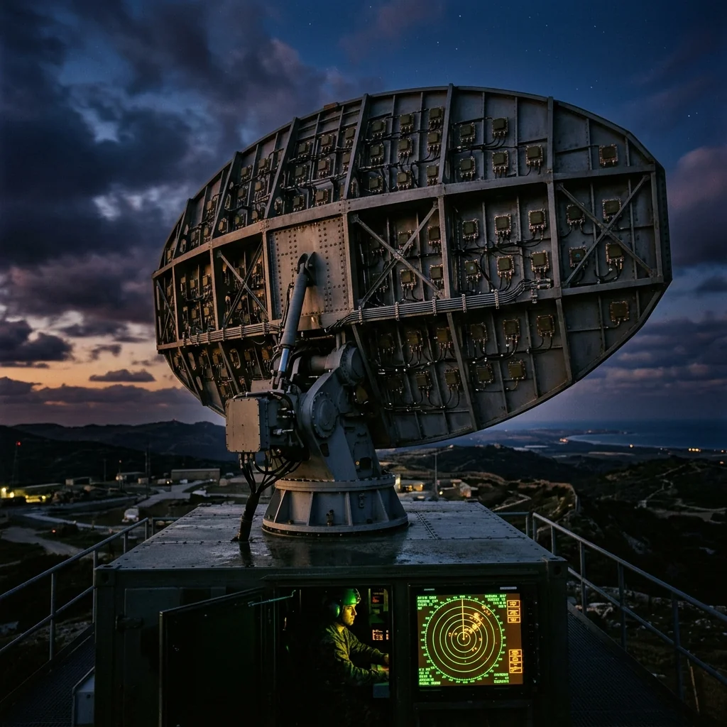
Early radar systems faced an uncomfortable trade-off. Fine range resolution required short pulses, but short pulses contain less energy than long ones. Less energy means weaker target echoes, which means shorter detection range. A radar designer could have range or resolution, but not both. Pulse compression eliminated that trade-off by encoding a long, high-energy pulse with internal modulation that can be collapsed into a short, high-resolution pulse in the receiver. The technique effectively decouples transmit energy from range resolution, and it has been the foundation of practically every military and commercial radar built since the 1960s.

The Fundamental Problem

A simple unmodulated radar pulse of duration τ has a range resolution of ΔR = cτ/2, where c is the speed of light. A 1 microsecond pulse resolves targets separated by 150 meters. To achieve 1.5-meter resolution, the pulse must be 10 nanoseconds long. But the energy in a pulse equals the peak power multiplied by the pulse duration: E = P_peak × τ. A 10 ns pulse at 1 kW peak power delivers only 10 microjoules of energy, which limits the maximum detection range to a few kilometers against a 1 m² target.

The solution is to transmit a long pulse (high energy) that has been internally modulated so that it occupies a wide bandwidth B. The range resolution is then determined by the bandwidth, not the pulse duration: ΔR = c/(2B). A 100 MHz bandwidth chirp provides 1.5-meter resolution regardless of whether the pulse is 1 microsecond or 100 microseconds long.

Linear Frequency Modulation: The Workhorse Waveform

The most common pulse compression waveform is the Linear Frequency Modulated (LFM) chirp. During the pulse, the instantaneous frequency sweeps linearly from f₀ to f₀ + B (up-chirp) or from f₀ + B to f₀ (down-chirp). The rate of frequency change is μ = B/τ Hz per second.

LFM is popular for several practical reasons:

• Doppler tolerance: LFM chirps are relatively insensitive to target Doppler shift. A Doppler offset shifts the compressed pulse in time (causing a small range error) but does not significantly degrade the compression quality. This makes LFM suitable for targets at all velocities.
• Simple generation: A voltage-controlled oscillator (VCO) driven by a linear ramp generates an LFM signal directly. Modern implementations use Direct Digital Synthesis (DDS) for precise, repeatable chirps.
• Matched filter simplicity: The matched filter for an LFM chirp is simply a conjugate-reversed copy of the chirp, which can be implemented as an analog Surface Acoustic Wave (SAW) device or a digital FIR filter.

Waveform Type	Compression Ratio	Doppler Tolerance	Sidelobe Level (unweighted)	Implementation
LFM (Linear Chirp)	100 - 100,000	Excellent	-13.2 dB	VCO, DDS, SAW
NLFM (Nonlinear Chirp)	100 - 10,000	Good	-30 to -50 dB	DDS, arbitrary waveform
Phase-coded (Barker)	13 (max)	Poor	-22.3 dB (Barker-13)	BPSK modulator
Phase-coded (Frank/P4)	N² (N = code length)	Moderate	-N (dB, approx)	Polyphase modulator
Stepped Frequency	N × per-step BW/total BW	Poor	-13.2 dB	Frequency synthesizer

The Matched Filter

The matched filter is the optimal linear filter for maximizing the signal-to-noise ratio (SNR) of a known signal in white Gaussian noise. For pulse compression, the matched filter's impulse response is the time-reversed, conjugated replica of the transmitted waveform. When the received echo passes through this filter, the output is the autocorrelation function of the transmitted waveform, which produces a narrow peak whose width is approximately 1/B.

Analog Implementation

In legacy radar systems, the matched filter was implemented using Surface Acoustic Wave (SAW) dispersive delay lines. The SAW device applies a frequency-dependent delay that is the inverse of the chirp slope, causing all frequency components to arrive at the output simultaneously, producing the compressed pulse. SAW filters are still used in some compact, low-power radar systems where digital processing resources are limited.

Digital Implementation

Modern radar receivers digitize the IF signal and perform matched filtering in an FPGA or DSP. The matched filter is typically implemented in the frequency domain using the overlap-save or overlap-add method: FFT the received data block, multiply by the conjugate of the reference chirp spectrum, and IFFT to produce the compressed output. For a radar with 100 MHz bandwidth and 10 μs pulses, this requires an ADC with at least 200 MS/s sample rate and 12 to 14 bits of resolution. The RF front-end components feeding the ADC, including LNAs, mixers, and IF filters, must maintain phase linearity across the full chirp bandwidth to preserve compression quality.

Range Sidelobes: The Unavoidable Artifact

The autocorrelation of a rectangular-envelope LFM chirp produces sidelobes at -13.2 dB relative to the main peak. These sidelobes are a direct consequence of the rectangular spectral shape of the chirp. In practical terms, a -13.2 dB sidelobe means that a strong target (like a building or ship) can mask a weaker target (like a small drone or swimmer) that is separated by just a few range cells.

Reducing sidelobes requires applying a weighting function (window) to the matched filter output or to the reference chirp spectrum before correlation. Common windows include:

Window	Peak Sidelobe (dB)	Main Lobe Width	SNR Loss (dB)	Typical Application
None (rectangular)	-13.2	1.0 × (1/B)	0	Maximum resolution
Hamming	-42.8	1.50 × (1/B)	1.34	General purpose
Taylor (-40 dB, n̄=5)	-40	1.33 × (1/B)	0.84	Surveillance radar
Chebyshev (-60 dB)	-60	1.65 × (1/B)	2.10	High-dynamic-range
Kaiser (β=6)	-44	1.42 × (1/B)	1.13	Adjustable sidelobe

The trade-off is always the same: lower sidelobes cost resolution (wider main lobe) and SNR (processing loss). The Taylor window is the preferred choice for most surveillance radars because it provides a nearly optimal trade-off between sidelobe level, main lobe width, and SNR loss. At RF Essentials, our waveguide terminations are used in radar transmitter test beds where precise power measurement is critical for validating the transmitted waveform quality before pulse compression processing.

Nonlinear FM: Built-In Sidelobe Control

An alternative to windowing is Nonlinear Frequency Modulation (NLFM), where the chirp rate varies across the pulse to create a non-rectangular spectral shape. By tapering the chirp rate at the beginning and end of the pulse (spending more time at the band edges), the spectrum approximates a Taylor or Hamming window shape without any post-processing loss. The compressed pulse of an NLFM waveform has inherently low sidelobes (typically -30 to -50 dB) with no SNR penalty beyond the slight reduction in effective bandwidth.

NLFM waveforms are more complex to generate and require precise frequency control, but modern DDS and arbitrary waveform generator technology makes them practical. Several current military radars use NLFM waveforms exclusively, eliminating the need for post-compression windowing and the associated resolution and SNR trade-offs.

Hardware Implications for the RF Chain

Pulse compression places specific demands on the radar's RF hardware that go beyond what a simple pulsed radar requires:

1. Transmitter amplitude flatness: The transmitter must maintain constant amplitude across the full chirp bandwidth. Amplitude ripple in the transmitted chirp creates paired echoes in the compressed output that mimic false targets.
2. Phase linearity: The transmitter and receiver chain must exhibit linear phase across the chirp bandwidth. Group delay variation of more than 1/(10B) seconds produces measurable sidelobe degradation.
3. Spurious signals: Any spurious frequency components within the chirp bandwidth create false targets in the range profile. The transmitter must maintain spurious-free dynamic range of at least 60 dBc across the chirp band.
4. ADC requirements: The ADC must sample at a rate of at least 2B (Nyquist), with sufficient bits to preserve the dynamic range of the compressed output. A PCR of 1,000 (30 dB) requires 5 additional effective bits beyond what the uncompressed dynamic range demands.
5. Wideband waveguide components: The waveguide bends, transitions, and couplers in the transmit and receive paths must maintain low VSWR and flat insertion loss across the full chirp bandwidth to preserve waveform fidelity.