Analog beamforming steers a beam by adjusting phase shifters in the RF hardware. It produces one beam at a time, in one direction, with one set of weights. Digital beamforming eliminates the analog phase shifters entirely. Instead, it digitizes the signal from every antenna element independently and forms beams in software. The result is the ability to form multiple simultaneous beams in arbitrary directions, adaptively null jammers, and reconfigure the array's spatial response on a pulse-by-pulse or symbol-by-symbol basis.
This article covers the signal processing principles, hardware architecture, and practical tradeoffs of digital beamforming for radar and communications phased arrays.
1. Analog vs. Digital vs. Hybrid
| Architecture | Beams | Adaptivity | Data Rate per Element | Cost per Element |
|---|---|---|---|---|
| Analog | 1 | None (fixed weights) | None (RF combining) | Low |
| Hybrid | Limited (# of digital channels) | Sub-array level | Moderate | Moderate |
| Full Digital | Unlimited (compute-limited) | Element level | High (ADC per element) | High |
The practical difference is flexibility. An analog array with 1,024 elements produces one beam. A digital array with 1,024 elements and full element-level digitization can simultaneously produce dozens of independent beams, each with independently optimized spatial filtering. For radar, this means tracking hundreds of targets simultaneously. For communications, this means serving hundreds of users in different directions on the same time-frequency resource.
2. Element-Level Digitization
In a digital beamforming system, each antenna element (or small sub-array of 2 to 4 elements) has its own receive chain: LNA, downconverter, and ADC. The ADC must sample the full signal bandwidth with sufficient dynamic range to capture both desired signals and jammers simultaneously.
The Data Firehose: A 256-element array with 14-bit ADCs sampling at 3 GSPS per element produces 256 x 14 x 3 x 10⁹ = 10.8 Tbps of raw data. This data must be transported from the array face to the digital processing backend via high-speed serial links (JESD204B/C) and processed in real time. The data transport and processing infrastructure is often more challenging (and expensive) than the RF front end itself.
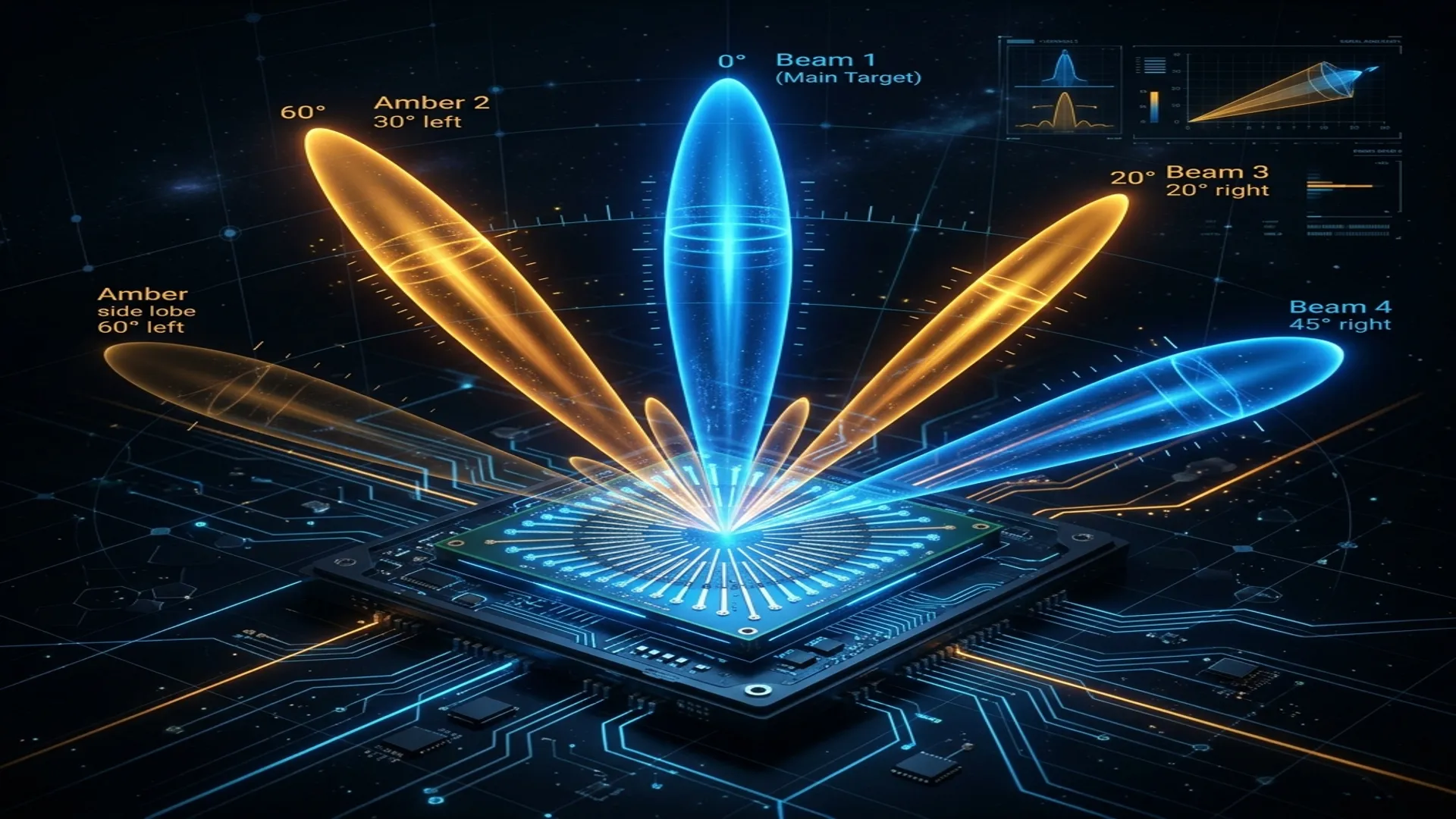
3. Digital Beam Synthesis
Once the element signals are digitized, beam formation is a weighted sum in the digital domain. For a linear array of N elements, the output of beam k is:
yk(t) = sum over n from 1 to N of: wk,n* xn(t)
where xn(t) is the digitized signal from element n and wk,n is the complex weight (amplitude and phase) applied to element n for beam k. Different weight vectors produce beams pointing in different directions. All beams are computed simultaneously from the same set of element data.
Steering a Beam
To steer a beam to angle theta from broadside, the weight for element n is: wn = exp(j 2pi n d sin(theta) / lambda), where d is the element spacing and lambda is the wavelength. This applies a linear phase gradient across the array that coherently combines signals arriving from direction theta.
4. Adaptive Nulling
The most powerful advantage of digital beamforming is adaptive nulling: the ability to automatically place nulls (zeros) in the array pattern at the directions of jamming or interference sources, without affecting the main beam pointing direction.
How It Works
- Detect: The processor identifies interference sources from the covariance matrix of the element signals.
- Compute: An adaptive algorithm (typically Sample Matrix Inversion or one of its variants: Loaded SMI, diagonal loading) computes a weight vector that minimizes the total interference power while maintaining gain in the look direction.
- Apply: The computed weights replace the conventional steering weights for the affected beam.
The number of independent nulls that a digital array can place equals N-1, where N is the number of independently digitized channels. A 64-channel digital array can theoretically null 63 independent jammers simultaneously.
5. Space-Time Adaptive Processing (STAP)
STAP extends adaptive nulling to joint spatial and temporal (Doppler) filtering. A conventional adaptive beamformer nulls interference at specific angles. STAP nulls interference at specific angle-Doppler combinations, which is essential for airborne radar where ground clutter appears at every angle with a Doppler shift determined by the platform velocity and look angle.
STAP requires the digital processing of NxM dimensions (N spatial channels x M temporal/Doppler samples), making it computationally intensive. Modern STAP implementations use reduced-rank techniques (eigenvalue decomposition, joint-domain localized processing) to make the computation tractable on FPGA and GPU hardware.
6. Hardware Implications
- ADC performance: Each element needs an ADC with sufficient SFDR (70+ dB) and bandwidth to capture the full signal and interference environment. GSPS-class ADCs with 12 to 16 bits are now available from ADI, TI, and Renesas.
- High-speed data transport: JESD204C serial links at 16+ Gbps per lane transport element data from the array to the processing backend.
- FPGA processing: Beamforming operations (complex multiply-accumulate for each beam, each element, each time sample) map efficiently onto FPGA DSP slices. A modern Xilinx Versal ACAP can form 16+ simultaneous beams from 256 elements in real time.
- RF front end quality: Digital beamforming amplifies any channel-to-channel mismatch (gain, phase, delay) across the array. The LNAs, downconverters, and anti-alias filters must be tightly matched, or digital calibration must compensate for the mismatches.
RF Essentials manufactures the passive waveguide and feed network components that connect antenna elements to the RF front end in phased array systems. Precision-matched components for minimal channel-to-channel variation.
Frequently Asked Questions
How does digital beamforming differ from analog beamforming?
Analog beamforming steers a beam with RF phase shifters, producing one beam at a time in one direction with one set of weights. Digital beamforming eliminates those phase shifters and digitizes the signal from every element independently, forming beams in software. A 1,024-element digital array can produce dozens of simultaneous independent beams, adaptively null jammers, and reconfigure its spatial response on a pulse-by-pulse or symbol-by-symbol basis.
What is adaptive nulling, and how many jammers can a digital array reject?
Adaptive nulling automatically places pattern zeros at interference directions without disturbing the main beam. The processor detects sources from the covariance matrix of the element signals, an adaptive algorithm such as sample matrix inversion computes weights that minimize interference power while holding gain in the look direction, and those weights replace the conventional steering weights. A digital array with N independently digitized channels can null up to N minus 1 independent jammers.
What is the main hardware challenge of full digital beamforming?
The data firehose. A 256-element array with 14-bit ADCs sampling at 3 GSPS per element produces roughly 10.8 terabits per second of raw data that must be transported over high-speed serial links like JESD204C and processed in real time on FPGAs. That transport and processing backend is often harder and more expensive than the RF front end itself, and any channel-to-channel gain or phase mismatch must be tightly matched or digitally calibrated out.